In this paper a statistical analysis of sporadic-E qsos in the 50 MHz
frequency band is presented. The data base comprises 979 records of approx.
550 amateur radio stations worked or heard by the author between 1983 and
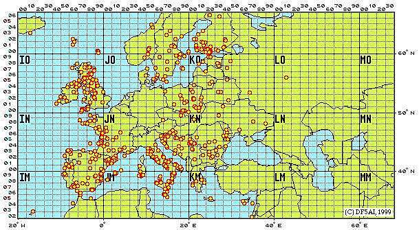
1999 from JO52CJ, JO31PG or JO40DF (figure 1).
 |
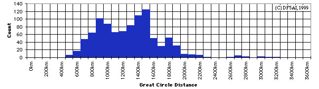 |
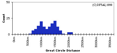
This distribution is somewhat unexpected: instead of having a single
maximum around 1400-1600 km, a number of peaks are obvious, i.e.
at 900 km, 1500 km and 1800 km. Thus, it appears that skips of a particular
distance are more likely than skips of any other distance, something which
is not predicted by the theory of sporadic-E.
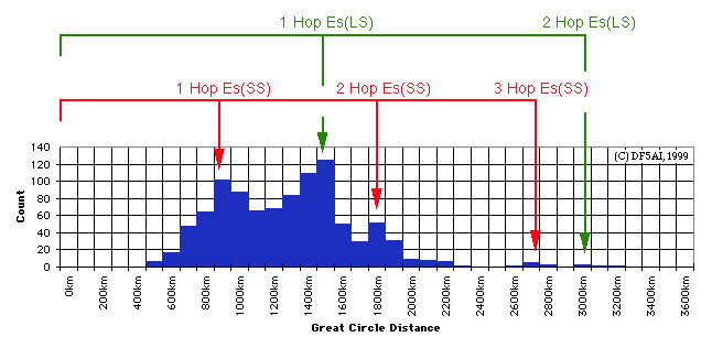
Nevertheless, all three maxima may still be interpreted in terms of
two propagation modes if multiple-hop propagation is taken into account:
figure 3 interprets the sporadic-E analysis in terms of multiple-mode/multiple-hop
propagation. The short-skip mode, Es(SS), generates the first peak at a
skip distance of approx. 950 km. The same mode also appears as a 2nd hop
at approx. 1800-1900 km. Finally the tripple-hop variant causes a third
peak at approx. 2700-2800 km. Because higher order hops occur less
often than lower order ones, the third peak is smaller than the second
and the second peak is smaller than the first. The long skip mode, Es(LS),
accounts for the maximum which appears at approx. 1500-1600 km. Its double-hop
variant also generates a small peak at 3000-3200 km, just above the three-hop
type of Es(SS).
 |
In a further analysis, the short-skip and the long-skip modes were isolated
from the database by selecting stations in the 800-1100km and 1300-1500km
ranges, respectively. The two data subsets were analysed independently,
as described in table 1.
| Analysis | Results |
| Season | Both the short-skip and the long-skip modes typically appear in the months of May to September/October. Both commence very abruptly in May, although occasional Es(LS) was found earlier. No Es(SS) or Es(LS) were observed in November and December. |
| Number of events | The number of events differs significantly when comparing the Es(SS) and Es(LS) mode. The frequency of Es(SS) is a smooth function of time i.e. the season starts in May, peaks slightly in June and fades out gently after that. This is not the case for Es(LS): the long-skip mode also commences abruptly in May but the number doubles in June. In this month Es(LS) occurs twice as frequently as Es(SS). In July and August the numbers of Es(LS) are almost identical, but are lower than in May. Very few events were found in September and October - this is also so for the short-skip mode. |
| Diurnal occurrence | Both modes, Es(SS) and Es(LS), have very similiar daily profiles. In particular, a daily peak exists in the late morning (9-11UT) and also in the early evening (17-19UT). However, there is very strong evidence that Es(LS) occurs one to two hours before the Es(SS) mode. |
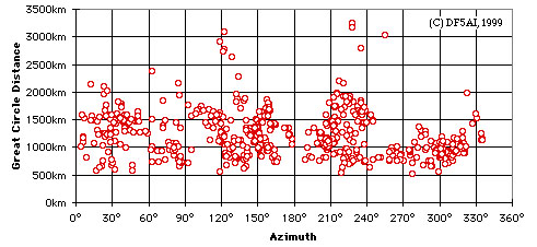
| Azimuth | Very often Es(SS) and Es(LS) propagation coexist with identical antenna headings. However, sometimes only one of the modes appears in a particular antenna direction. |
| Geography | No distinct geographical distribution of Es(SS) and Es(LS) was found. |
The long-skip mode appears to be in agreement with the dxers´ sporadic-E expectations. However, the short-skip mode, Es(SS), is disturbing because the short distance (e.g. 700-900km) requires a relatively high penetration angle into the E-layer (elevation approx. 10-12 degrees) and this would be associated with a surprisingly high electron density. This is true when Es(SS) originates at the same height as Es(LS), i.e. in approx. 100-110 km. However one might speculate that short-skip propagation corresponds to a lower scattering height of around 80-90km. In fact, strong vhf radio echos from the mesosphere have been reported but forward scattering in the mesosphere at low antenna elevation would, however, be a new phenomenon.
Statistical data was insufficient for an evaluation of an equivalent
range gate analysis for 144 MHz sporadic-E. However, preliminary results
indicate a different behaviour for 144 MHz. In particular there is evidence
that the major peak appears at longer distances and that the other peaks
are less pronounced than in 50 MHz sporadic-E.
Possible sources of error
In order to rule out contamination of the statistical data, possible
sources of error were analysed (table 2).
| Possible error | Summary |
| Too few statistical data | In the 1999 sporadic-E season, the number of records grew
from approx. 650 to almost 1000 and, consequently, the distribution function
stabilized. Even when dealing with much less data, results similiar to
those in figure 2 were obtained. In the case of the 1998 sporadic-E season,
for example, a multi-peak distribution function with peaks at similar distances
was also found although only 165 stations were monitored (figure 4).
Hence there is strong evidence that figure 2 is not distorted by too few
data.
Figure 4. Range gate analysis of 50 MHz sporadic-E in 1998. |
| Topographical features | Local topographical features, such as hilly terrain, may
cut off low antenna elevation and may, therefore, reduce the level of long
distance propagation. However this is not the case here as 1) similiar
distributions were found at two locations, JO31PG and JO40DF, and 2) the
correlation of skip-distance and local antenna azimuth did not indicate
any cutoff effects or preferred antenna directions (figure 5). Hence it
is very unlikely that the distribution shown in figure 2 is a consequence
of local terrain effects.
Figure 5. Sporadic-E skip distance versus local azimuth. |
| Continental shape | The continental shape of Europe might also affect the range
gate analysis. If, for example, sea water terrain would dominate a particular
range gate, a corresponding minimum would occur in the distribution. In
order to analyse this possible effect, each of the Maidenhead grid locators
in Europe was characterized according to its dominant terrain type, i.e.
land, sea or coastal terrain. In a second step, a range gate analysis was
calculated which included all European grid squares. The resulting distribution
indicated the land and sea areas as a function of distance from the oberserver's
location (figure 6). No correlation between continental shape and number
of amateur radio stations was found, so that figure 2 may be assumed
free from this possible error.
Figure 6. Sea, land and coastal terrain areas as a function of distance in reference to JO40DF. |
| Geographical density of radio amateurs | The range gate analysis could be affected by an inhomogenous
distribution of radio amateur stations. One could speculate that the first
peak in figure 2 is a consequence of the large number of British 6m-operators.
Exclusion of all stations located in this IO-square i.e. Great Britain
and Ireland, resulted in a decrease in the magnitude of the 900 km peak,
but did not remove the peak altogether (figure 7). The geographical density
of 6m-operators may, nevertheless, influence the results shown in figure
2; only further observations from different locations can clarify this
point.
Figure 7. Range gate analysis similiar to figure 2 excluding stations located in the IO square. |
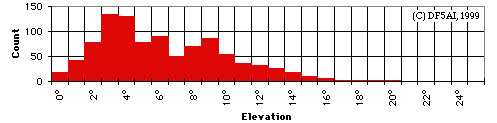
| Vertical antenna pattern | Unwanted or unexpected side lobes in the H-plane antenna
pattern may filter out particular elevation angles and so bias the communication
range of a radio station. In order to investigate this possibility, the
antenna elevation of each of the 979 records was calculated: for example,
10 degree elevation corresponds to qsos in the 920-930 km range (height
of scatter volume: 105 km). It was found that each of the stations was
definitely captured by the antenna's main lobe (figure 8). Finally, different
antennas were used by DF5AI (yagi as well as wire antenna) and all arrays
provided results similiar to those of figure 2. Hence it is believed that
the vertical antenna pattern only plays a minor role in figure 2.
Figure 8. Calculated elevation profile (979 records, scatter height 105 km). |
This work should encourage other radio amateurs to analyse their personal
qso databases in a similiar fashion with the aim of investigating a possible
unknown propagation mode:
Do other radio amateurs confirm the existence of a double- or tripple-peak
distribution function similiar to figure 2?
If yes, what is the distance at which the maxima appear?
What results are obtained when analysing 144MHz sporadic-E?